Fine Tuning Your Objects - Dimension & Expression Attributes

Most of the time, clients simply care about getting their data.   And it is sometimes no small effort to transform business requirements (or lack thereof) into a working QlikView application.  Sometimes there is no room left in the budget for the finer design points. 

But many times, I find that going that extra mile to bring simple and intuitive meaning to the data can make the difference between QlikView being perceived as a lackluster business tool and the “lean forward experience” that we all want it to be (to use the words of Donald Farmer). 

Maybe we should highlight the new product line in our bar chart, or maybe we want to see the best and worst performers in a table or I want my forecast as a dotted line and my average trend to be a thinner line.

Now this kind of highlighting is not always intuitive in QlikView.  It took me a while to realize the power of these settings and I am still not at the point where I have memorized all the small syntax pieces needed to add these touches.  So I thought I would put together a small article to illustrate some examples and also to give myself and others an easy place to reference these codes.

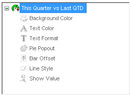
The items we will cover are accessible in the dimensions and expressions tabs of your object properties.  If you expand the plus sign in your used dimensions or expressions, you will find the attributes we are discussing.  All these settings will require some form of calculated expression to work.  Also note that these settings will override any other display settings you have in the object.  We will examine these attributes in order.

 

Dimension Attributes

Dimension attributes only work in straight or pivot tables and will affect dimension columns.

Background Color and Text Color

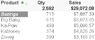
These two attributes work the same way with one affecting the cell background and the other affecting the font color.  In this case, we want to highlight our new product line:

Background Color:

=IF(Product='Bazinga',RGB(100,100,100))

Text Color:

=IF(Product='Bazinga',White()) 

    

Text Format

The Marketing Director likes that but wants to go  a step further by displaying the text in bold italics.  No problem:

Text Format:

=IF(Product='Bazinga','<I><B>')

 

Note that you can use the following text formats and also that you can use more than one at a time like in our above example.

=’<B>’	Bold
=’<I>’	Italics
=’<U>’	Underline

Expression Attributes

Expression attributes are available in some capacities for all chart types.  These attributes affect the expression columns of a chart.

Background Color, Text Color and Text Format

Just like in the dimension attributes, Background and Text color change the colors of values in the data.  Text color only has an effect on straight or pivot tables.  Background color is adjustable for tables, and several other charts.  First, let’s adjust our straight table example again.  This time we want to highlight the cells that represent the best and worst performers in their expression columns.  We will also adjust the text format:

Background Color:

=IF(RANK(SUM({<IsForecast={0}>}Qty))=1,LightGreen(),
                IF(RANK(-SUM({<IsForecast={0}>}Qty))=1,Red()))

Text Color:

=IF(RANK(-SUM({<IsForecast={0}>}Qty))=1,White())

Text Format:

=IF(RANK(SUM({<IsForecast={0}>}Qty))=1,'<B>')

Now let’s look at a bar chart.  We will go back to our previous example of highlighting the value that is our featured product type.  This is done with the Background Color attribute:

Background Color:

=IF(Product='Bazinga',RGB(0,255,0))

Pie Popout

The Pie Popout attribute is obviously only available when using a pie chart.  This will advance one slice of the pie slightly out from the center.  Let’s highlight our chosen product line.

Pie Popout:

Product='Bazinga'

Bar Offset

This attribute, when used in a bar chart, will raise a bar off the x-axis by a calculated amount.  This could be useful to create gaant charts.  For lack of a better example, we will stack each year’s sales on top of the previous total.

I first created an invisible expression called RunningTtl:

IF(RowNo()=1,SUM(Sales),
                ABOVE(RunningTtl)+SUM(Sales))

Then I created this expression in the Bar Offset attribute:

IF(RowNo()=1,SUM(Sales),
                ABOVE(RunningTtl)+SUM(Sales))-SUM(Sales)

Line Style and Show Value

These attributes are for use in line charts (or combo charts with line expressions).  The Line Style attribute changes the line to dotted, for example.  Show Value will allow us to selectively choose which points have a textual representation.  As stated before, these attribute settings will override any higher level configurations.  This time, we would like the sales figures to be represented by a continuous line (default) and the forecast to be displayed as a dotted line.  We also have a request to label the current year’s sales with text.  In addition, we want an average line that is very thin compared to the sales line:

Line Style (continuous vs. dotted):

=IF(IsForecast=1,'<S3>')

Show Value:

Year=Year(Today())

Line Style (width):

='<W.5>'

Line Style – Type	Description
=’<S1>’	Continuous
=’<S2>’	Dashed
=’<S3>’	Dotted
=’<S4>’	Dotted & Dashed

Line Style – Width	Description
=’<Wn>’	n = .5 – 8 to determine width of the line.

I am sure there are many more compelling uses for these attributes.  I believe they can add tremendous value in your visualizations as long as they are used for valid reasons.  Take your applications to the next level.